Learnability and VC Dimension

Table of contents

1. Overview
2. Motivation
3. Learnability
   1. Realizability
   2. $\epsilon$ - $\delta$ Parameters
   3. Finite Hypothesis Class
   4. PAC Learnability
   5. Agnostic PAC-Learnability
   6. Uniform Convergence implies Agnostic PAC Learnability
4. VC Dimension
5. Fundamental Theorem of Learnability

Overview

In this lecture, we will discuss learnability and show when the Empirical Risk Minimization methods that we’ve introduced will succeed. We will start our discussion from simple settings under strong assumptions, realizability and infinite hypothesis class. We will define formally PAC-Learnability and generalize our conclusion to settings where realizability does not hold and where the class is infinite. The concept of VC-dimension will be introduced to quantify the power of infinite hypothesis classes. Finally, we will reach the fundamental theorem of statistical learning.

Motivation

In our previous discussion, we introduced the empirical risk minimization (ERM) method as an approximation to the true risk minimization and we also introduced different ways to restrict our hypothesis class so that our classifiers found by minimizing ERM can have better performance on unseen data. We saw a theoretic analysis on Logistic Regression and Naive Bayes in Classification Fundamentals. In this lecture, we want to generalize the discussion to the entire ERM methods and try to answer some fundamental questions related to the concept of learning.

First of all, we haven’t had a clear definition of what does it mean to be able to learn, and need to answer that. We also want to ask, what hypothesis class should we choose and what limitations do different hypothesis classes have. Further more, given a hypothesis class, we would like to discuss and determine what kinds of learning rules should we use, and how many data points do we need to learn a good model. With these questions in mind, we will start our discussion from simple settings and then try to generalize our conclusions.

Learnability

Realizability

We start our discussion with a simplifying assumption, realizability. Formally, realizability means that there exists an optimal hypothesis \(h^*\in \mathcal{H}\) such that the true risk $L_{\mathbb{P}(h^*)}=0$.

This is a strong assumption and it implies that with probability $1$, over random samples $S \sim \mathbb{P}$, $L_S(h^*)=0$

However, this strong assumption only implies the existence of such a hypothesis that can give $0$ error, it is not guaranteed that the particular hypothesis $h_S$ found by minimizing any ERM is the optimal hypothesis $h^*$. The realizability assumption makes sure our hypothesis class is “rich” or “capable” enough, so that we don’t need to worry about under-fitting, but we can still be overfitting by only minimizing the empirical error. Thus, we want to further discuss that under this assumption, what is the risk of the ERM hypothesis $h_S$ on the unseen data and can this risk be bounded such that we are guaranteed to find a good hypothesis?

$\epsilon$ - $\delta$ Parameters

To quantitatively measure how good our hypothesis is, we introduce the $\epsilon$ and $\delta$ parameters for our discussion. The $\epsilon$ parameter is called accuracy parameter and is used to quantify the quality of the prediction. Concretely, we interpret the event $L_\mathbb{P}(h_s) > \epsilon$ as a failure of the learner, while if $L_\mathbb{P}(h_S) \leq \epsilon$, we view the output of the ERM as an approximately correct hypothesis.

However, this single parameter is not enough because $h_S$ depends on the training set $S$, and the training set is picked by a random process so that there is randomness in the result of the ERM. It is not realistic to expect that with full certainty $S$ will suffice to direct the learner toward a good hypothesis, as there is always some probability that the sampled training data happens to be very non-representative of the underlying distribution $\mathbb{P}$. We therefore denote the probability of getting a non-representative sample by $\delta$, and call $(1-\delta)$ the confidence parameter of our prediction.

Finite Hypothesis Class

To bound the error of the ERM hypothesis $h_S$, we further introduce some restrictions on the hypothesis class $\mathcal{H}$ so that we can prevent overfitting. The simplest type of restriction on a class is imposing an upper bound on its size, that is, the hypothesis class $\mathcal{H}$ has a finite cardinality. With this additional assumption, we can show that the ERM hypothesis will not overfit, i.e., have a bounded error on unseen data.

Let $\mathcal{H}$ be finite. Let $\delta \in (0,1)$, $\epsilon >0$ and $N \geq \frac{\log(|\mathcal{H}|/\delta)}{\epsilon}$. Then, for any distribution $\mathbb{P}$ for which realizability holds, we probability at least $1-\delta$ over the choice of dataset $S$ of size $N$, every ERM hypothesis $h_S$ satisfies $L_\mathbb{P} \leq \epsilon.$

Let \(\mathcal{H}_B\) be the set of “failed” hypotheses, that is \(\mathcal{H}_B = \{ h \in \mathcal{H}: L_\mathbb{P}(h) > \epsilon\}.\) In addition, let $M$ be the set of misleading samples, that is \(M = \{ S : \exists h \in \mathcal{H}_B, L_S(h)=0 \}\) Namely, for every $S \in M$, there is a ’failed’ hypothesis, $h \in \mathcal{B}$, that looks like a ’good’ hypothesis on $S$.

Now, recall that we would like to bound the probability of the event $L_\mathbb{P}(h_S)>\epsilon$. Since the realizability implies that $L_S(h_S)=0$, it follows that the event \(L_\mathbb{P}(h_S)>\epsilon\) can only happen if for some \(h\in \mathcal{H}_B\), we have $L_S(h) =0$.

In other words, the failure will only happen if our training data is in the set of misleading samples Set $M$. Formally, we have \(\{S : L_{\mathbb{P}}(h_S)>\epsilon\} \subseteq M\) As we can write $M$ as \(M = \cup_{h \in \mathcal{H}_B}\{S : L_{S}(h)=0\}\) Hence, \({P}\left( \{ S: L_\mathbb{P} (h_{S}) > \epsilon \}\right) \leq {P}\left( \cup_{h \in \mathcal{H}_B}\{S : L_{S}(h)=0\}\right)\) Applying the union bound to the right-hand side yields \({P}\left( \{ S: L_\mathbb{P} (h_{S})\right) \leq \sum_{h \in \mathcal{H}_B} {P} \left(\{S : L_{S}(h)=0\}\ \right)\) Next, we can bound each summand of the right-hand side. Fix some ’failed’ hypothesis \(h \in \mathcal{H}_B\), the event $L_S(h) =0$ is equivalent to the event that in the training set, $\forall i$, $h(x_i)=y_i$. Since the training data are i.i.d. sampled, we have \({P} \left(\{S : L_{S}(h)=0\}\ \right) = \prod_{i=1}^N {P} \left( \{x_i: h(x_i) = y_i\} \right)\) For each individual sampling of an element of the training set, we have \({P} \left( \{x_i: h(x_i) = y_i\} \right) = 1-L_{\mathbb{P}}(h) \leq 1-\epsilon\) where the last inequality follows from the fact that \(h \in \mathcal{H}_B\).

Using the inequality $1-\epsilon \leq e^{-\epsilon}$, we have for every \(h \in \mathcal{H}_B\), \(P\left( S: L_{S}(h) = 0\right) \leq (1-\epsilon)^N \leq e^{-\epsilon N}\)

Therefore, we have \(P\left( S: L_{\mathbb{P}}(h_S) > \epsilon \right) \leq |\mathcal{H}_B| e^{-\epsilon N} \leq |\mathcal{H}|e^{-\epsilon N}\) Let $\delta = P\left( S: L_{\mathbb{P}}(h_S) > \epsilon \right)$, we will reach the desired conclusion that with probability at least $1-\delta$, and having $N \geq \frac{\log (|\mathcal{H}|/\delta)}{\epsilon}$, \(L_{\mathbb{P}}(h_S) \leq \epsilon.\)

A weaker result can be proved without realizability, see Exercise 2 for details.

PAC Learnability

We see that the finite hypothesis class makes it possible to bound the unseen error of ERM hypothesis. In order to generalize this result, we first give a formal name of such hypothesis classes. As we are using the $\epsilon$ and $\delta$ parameters which implies the conclusion is both approximate and not determined, we use the name Probably approximately correct learnability, also known as PAC-Learnability. A formal definition is as follows,

(PAC-Learnability). Assuming realizability, a hypothesis class $\mathcal{H}$ is PAC-learnable if there exists a function $N_\mathcal{H}(\epsilon, \delta)$ and a learning algorithm with the following property: For every $\epsilon, \delta \in (0,1)$ and every distribution $\mathbb{P}$, training using $N \geq N_\mathcal{H}(\epsilon, \delta)$ i.i.d. samples generated from $\mathbb{P}$, the learning algorithm returns a hypothesis $h$ such that $L_\mathbb{P} \leq \epsilon$ with confidence $(1-\delta)$ over choice of samples.

Informally, PAC-learnability of class $\mathcal{H}$ means that enough number of random examples drawn from the data distribution will allow approximate risk minimization, i.e., ensure $L_\mathbb{P}(h) \leq \epsilon$ with probability $\geq 1-\delta$, where the number of samples needed depends on the desired tolerances $(\epsilon, \delta)$.

Note here $\epsilon$ and $\delta$ are inevitable. $\delta$ arises due to the randomness of training data $S$ drawn from $\mathbb{P}$ and $\epsilon$ arises due to the actual hypothesis picked by the learner on the finite data $S$.

With this formal concept of PAC-learnable defined, we can discuss the situations when our two assumptions on realizability and finite hypothesis class do not hold. Concretely, is the hypothesis class still learnable if realizability does not hold? And on the other hand, what about infinite hypothesis classes? Are they PAC-learnable?

Agnostic PAC-Learnability

We first release the realizability assumption. By No-Free-Lunch (NFL) theorem, we know that no learner is guaranteed to match the Bayes classifier in general, as there’s always an adversarial distribution that can be constructed on which our learner fails while another may succeed. Thus, if the realizability does not hold, we don’t have any hope of satisfying $L_{\mathbb{P}} \leq \epsilon$.

We now can only weaken our aim, and see if we can at least come $\epsilon-$ close to the best possible classifier within our hypothesis class with high probability, i.e. \(L_{\mathbb{P}}(h_S) \leq \inf_{h' \in \mathcal{H}} \mathbb{P}(h') + \epsilon.\) In this setting, the hypothesis class $\mathcal{H}$ may be bad, but we can still try to be approximately as good as the best possible hypothesis within this class. This weaker property is known as Agnostic PAC-Learnability.

(Agnostic PAC-Learnability). A hypothesis class $\mathcal{H}$ is agnostic PAC learnable if there exist a function $N_\mathcal{H}: (0,1)^2 \to N$ and a learning algorithm with the following property: For every $\epsilon, \delta \in (0,1)$ and for every distribution $\mathbb{P}$ over $\mathcal{X} \times \mathcal{Y}$, when running the learning algorithm on $N>N_\mathcal{H}(\epsilon, \delta)$ i.i.d. samples generated by $\mathbb{P}$, the algorithm returns a hypothesis $h$ such that, with probability of at least $1-\delta$ over the choice of the $N$ training samples, $$L_{\mathbb{P}}(h) \leq \inf_{h' \in \mathcal{H}} \mathbb{P}(h') + \epsilon.$$

Clearly, if the realizability assumption holds, Agnostic PAC-Learnability provides the same guarantee as PAC-Learnability. In that sense, Agnostic PAC-Learnability generalizes the definition of PAC-Learnability. When the realizability assumption does not hold, no learner can guarantee an arbitrarily small error. Nevertheless, under the definition of Agnostic PAC learning, a learner can still declare success if its error is not much larger than the best error achievable by a predictor from the class $\mathcal{H}$. This is in contrast to PAC Learning, in which the learner is required to achieve a small error in absolute terms and not relative to the best error achievable by the hypothesis class.

We call decompose the error into the approximation error term and the estimation error term, where \(L_\mathbb{P}(h_S) = \epsilon_{apx} + \epsilon_{est}\) where \(\epsilon_{apx} := \min_{h\in \mathcal{H}}L(h)\) and \(\epsilon_{est} := L_\mathbb{P}(h_S) -\epsilon_{apx}.\)

As the approximation error depends on the fit of our prior knowledge via the inductive bias to the unknown underlying distribution, it won’t be minimized further more after we’ve chosen the hypothesis class $\mathcal{H}$. The Agnostic PAC-Learnability loosens the bound on this term but bound the estimation error uniformly over all distributions for a given hypothesis class.

Uniform Convergence implies Agnostic PAC Learnability

How can we make sure the ERM solution is close the true risk? One strong assumption one can make is that $L_S(h)$ for all $h \in \mathcal{H}$ is close to the true risk $L_\mathbb{P}(h)$, then the ERM solution $h_S$ will also have small true risk $L_\mathbb{P}(h_S)$. Hence, we introduce the notion of an $\epsilon-$representative data sample

($\epsilon$-representative). A dataset $S$ is called $\epsilon$-representative if $$\forall h \in \mathcal{H}, \quad |L_S(h) - L_\mathbb{P}(h)| \leq \epsilon.$$

The next simple conclusion we can make is that whenever the sample is $\epsilon/2$-representative, the ERM learning rule is guaranteed to return a good hypothesis.

Assume $S$ is $\epsilon/2$ - representative. Then, any ERM solution $h_S \in \argmin_{h \in \mathcal{H}} L_S(h)$ satisfies $$L_{\mathbb{P}} \leq \min_{h\in \mathbb{H}} L_{\mathbb{P}} + \epsilon.$$

For every $h\in \mathcal{H}$, $$\begin{aligned} L_{\mathbb{P}} & \leq L_S(h_S) + \epsilon/2 \\ & \leq L_S(h) + \epsilon/2 \\ & \leq L_{\mathbb{P}}(h) + \epsilon/2 + \epsilon/2 \\ & = L_{\mathbb{P}}(h) + \epsilon \end{aligned}$$

The simple theorem implies that to ensure that the ERM rule is Agnostic PAC-Learnable, it suffices to show that with probability of at least $1 - \delta$ over the random choice of a training set, it will be an $\epsilon$-representative training set. The following uniform convergence condition formalizes this requirement.

(Uniform Convergence). A hypothesis class $\mathcal{H}$ has the uniform convergence property w.r.t a domain $Z$ and a loss function $\ell$, if there exists a function $N_\mathcal{H}^{UC}: (0,1)^2 \to \mathbb{N}$ such that for every $\epsilon, \delta \in (0,1)$ and for every probability distribution $\mathbb{P}$ over $Z$, if $S$ is a sample of $N \geq N_\mathcal{H}^{UC}(\epsilon,\delta)$ i.i.d. examples drawn from $\mathbb{P}$, then, with probability of at least $1-\delta$, $S$ is $\epsilon$-representative.

Similar to the definition of sample complexity for PAC learning, the function $N_\mathcal{H}^{UC}$ measures the minimal sample complexity of obtaining the uniform convergence property, namely, how many examples we need to ensure that with probability of at least $1-\delta$ the sample would be $\epsilon$-representative. The term uniform here refers to having a fixed sample size that works for all members of $\mathcal{H}$ and over all possible probability distributions over the domain. The following corollary follows directly from the previous theorem and the definition of uniform convergence.

**Corollary**: If a class $\mathcal{H}$ has the uniform convergence property with a function $N_{\mathcal{H}}^{UC}$ then the class is Agnostically PAC learnable with the sample complexity $N_\mathcal{H}(\epsilon, \delta) \leq N_{\mathcal{H}}^{UC}(\epsilon/2, \delta)$.

VC Dimension

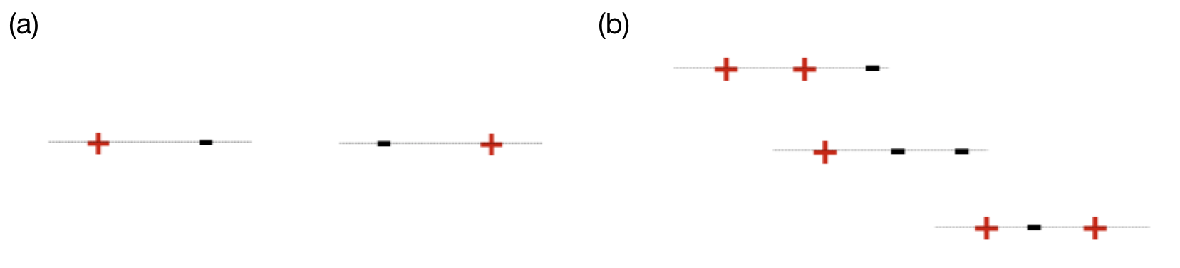
Now, let’s move to the situation of infinite hypothesis class. Clearly, we don’t have a measurement for the size of the hypothesis class any more, but it is still possible to quantitatively measure complexity of the model. For learnability in classification problems, what really matters is not the literal size of the hypothesis class, but the maximum number of data points that can be classified exactly. Take the simple situation in Figure 1 for example, the hypothesis class of 1-dimensional linear classifier has an infinite size, but this doesn’t mean this class is a very complex class. As shown in Figure 1 (a), two points with whatever labels can be classified correctly by a linear classifier, but in Figure 1 (b), we can see that this no longer holds for 3 points, as the last example in (b) cannot be classified correctly by any hypothesis in the linear classifier class. This inspires us that in order to measure the richness of our hypothesis class, we can try to construct a subset $C$ of the data domain for which our classifier fails or succeeds. To understand the power of our hypothesis class, we just focus on its behavior on $C$ and try to check how many different possible classification decisions on $C$ can our hypothesis class capture. Then, if the hypothesis class can explain all decisions possible on $C$, then one can construct a ’misleading data distribution’ so that we maintain realizability on $C$ but can be totally wrong on the part outside of $C$ and thus suffer large risk. This implies that to achieve learnability, we need to restrict the size of $C$.

Linear classifiers in 1D can shatter 2 points as in (a), but cannot classifier the last case correctly in (b). Thus the VC-Dimension of 1-D linear classifiers is 2.

To be more formal, here we introduce the definition of restriction of $\mathcal{H}$ to $C$ and the following definition of shattering and VC-Dimension.

Let $\mathcal{H}$ be a class of functions from $\mathcal{X}$ to $\{0,1\}$ and let $C=\{c_1,...,c_m\} \subset \mathcal{X}$. The restriction of $\mathcal{H}$ to $C$ is the set of functions from $C$ to $\{0,1\}$ that can be derived from $\mathcal{H}$. That is, $$\mathcal{H}_C=\{(h(c_1),...,h(c_m)): h \in \mathcal{H} \}$$ where we present each function from $C$ to $\{0,1\}$ as a vector in $\{0,1\}^{|C|}$.

If the restriction of $H$ to $C$ is the set of all functions from $C$ to ${0,1}$, then we say $\mathcal{H}$ shatters the set $C$, formally

(Shattering). A hypothesis class $\mathcal{H}$ shatters finite set $C \subset \mathcal{X}$ if the restriction of $\mathcal{H}$ to $C$ is the set of all functions from $C$ to $\{0, 1\}$. That is, $|\mathcal{H}_C| = 2^ {|C|}$.

With the idea of shattering in, we are now ready to present the definition of VC dimension.

(VC-dimension). The VC-dimension of a hypothesis class $\mathcal{H}$, denoted $VC-dim(\mathcal{H})$, is the maximal size of a set $C \subset \mathcal{X}$ that can be shattered by $\mathcal{H}$. If $\mathcal{H}$ can shatter sets of arbitrarily large size, we say that $\mathcal{H}$ has infinite VC-dimension.

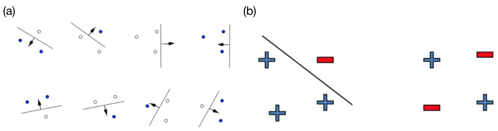
Here we give another example on 2-D linear classifiers, as shown in Figure 2. In (a), we can see that the linear classifier class can shatter 3 points in 2 dimensional space, however in (b), it cannot shatter 4 points as there exists a case where no linear classifier can correctly classifier the 4 points with the particular labelling as in the right figure in (b). This shows that the VC-Dimension of 2-D linear classifiers is 3.

Linear classifiers in 2D can classifier 3 points with arbitrary labelling as shown in (a), but cannot classifier 4 points correctly as in (b). Thus the VC-Dimension of 2-D linear classifiers is 3.

From this kind of observation, we can see that to show that $VC-dim(\mathcal{H})=d$, we need to prove two things:

1. There exists a set $C$ of size $d$ that is shattered by $\mathcal{H}$, this proves $VC-dim(\mathcal{H})\geq d$

2. No set of size $d+1$ is shattered by $\mathcal{H}$, this proves $VC-dim(\mathcal{H}) < d+1$. Thus $VC-dim(\mathcal{H})=d$.

Though we showed the VC-Dimension of $d$-dimensional linear classifier is $d+1$, most of the time, we can only have lower/upper bound of VC dimension, but not an exact computable number. Thus, it is important to understand the meaning of the lower and upper bound of VC-Dimension.

Fundamental Theorem of Learnability

As the name suggests, a pretty important theorem:

Let $\mathcal{H}$ be a hypothesis class of functions from a domain $\mathcal{X}$ to ${0, 1}$ and let the loss function be the $0 - 1$ loss. Then the following are equivalent:

1. $\mathcal{H}$ has the uniform convergence property.
2. Any ERM rule is a successful agnostic PAC learner for $\mathcal{H}$.
3. $\mathcal{H}$ is agnostic PAC learnable.
4. $\mathcal{H}$ is PAC learnable.
5. $\mathcal{H}$ Any ERM rule is a successful PAC learner for $\mathcal{H}$.
6. $\mathcal{H}$ has a finite VC-dimension.

In our previous discussion, we saw $1 \to 2$. $2 \to 3$, $3 \to 4$ and $2 \to 5$ are all trivial. For $4 \to 6$ and $5 \to 6$, there is detailed proof in [SSS] through the no-free-lunch theorem. Here, we take a closer look at $6 \to 1$, that a finite VC-dimension implies the uniform convergence property, and therefore is PAC-learnable. The detailed proof can be found in chapter 6 of [SSS], here we provide a high level sketch of the proof.

The two main parts of the proof are:

1. If $VC-dim(\mathcal{H})=d$, when restricting to a finite subset $C$ of the data domain, its effective size $|\mathcal{H}_C|$ is only $O|C|^d$, instead of exponential in $|C|$

2. Finite hypothesis class can be proved to have the uniform convergence property by a direct application of Hoeffiding inequality plus the union bound theorem. Similarly, the uniform convergence holds whenever the “effective size” is small.

To define the term “effective size”, we introduce the definition of Growth Function:

(Growth Function). Let $\mathcal{H}$ be a hypothesis class. Then the growth function of $\mathcal{H}$, denoted $\tau_\mathcal{H}: \mathbb{N} \to \mathbb{N}$, is defined as $$\tau_\mathcal{H}(N) = \max_{C \subset \mathcal{X}: |C|=N}|\mathcal{H}_C|$$

In words, $\tau_{\mathcal{H}}(N)$ is the number of different functions from a set $C$ of size $N$ to ${0, 1}$ that can be obtained by restricting $\mathcal{H}$ to $C$. We then can prove the Sauer’s lemma that can bound this growth function

**Lemma 13**. *Let $\mathcal{H}$ be a hypothesis class with $VC-Dim(\mathcal{H}) \leq d < \infty$. Then for all $N$, $\tau_\mathcal{H}(N) \leq \sum_{i=0}^d \begin{pmatrix} N\\i \end{pmatrix}$. In particular, if $N > d+1$ then $\tau_\mathcal{H}(N) \leq (eN)^d$*

Thus, finite VC-dimension implies polynomial growth, while infinite VC-dim means exponential growth. Intuitively, for any $C$ as a subset of $\mathcal{X}$, let $B$ be a subset of $C$ such that $\mathcal{H}$ shatters $B$.

Then,\(|\mathcal{H}_C| \leq \# \{ B \subset C: \mathcal{H} \text{ shatters } B \}\). That is, if $\mathcal{C}$ is the collection of subsets of $C$ that are shattered by $\mathcal{H}$, then $|\mathcal{H}_C|$ is upper-bounded by the cardinality of $\mathcal{C}$. Then we can show the ERM error is bounded using the growth function.

Let $\mathcal{H}$ be a class and $\tau_{\mathcal{H}}$ its growth function. Then for every distribution $\mathbb{P}(X,Y)$ and every $\delta \in (0, 1)$, with probability at least $1-\delta$ over the choices of $S \sim \mathbb{P}$, we have

\[|L_S(h) - L_\mathbb{P}(h) | \leq \frac{4+\sqrt{\log \tau_{\mathcal{H}}(2N)}}{\delta \sqrt{2N}}\]

And it follows from here that if VC-Dim($\mathcal{H}$) is finite, then the uniform convergence property holds, and indeed, \(N_{\mathcal{H}}^{UC}(\epsilon, \delta) \leq O(\frac{d}{(\delta \epsilon)^2})\) suffices for the uniform convergence property to hold.

A more quantitative version of this theorem is as follows, and the proof can be found in Chapter 28 of [SSS].

Let $\mathcal{H}$ be a hypothesis class of functions from a domain $\mathcal{X}$ to ${0, 1}$ and let the loss function be the $0 -1$ loss. Assume that $VC-Dim(\mathcal{H}) =d < \infty$. Then, there are absolute constants $C_1$, $C_2$ such that:

1. $\mathcal{H}$ has the uniform convergence property with sample complexity \(C_1\frac{d+\log(1/\delta)}{\epsilon^2} \leq N_\mathcal{H}^{UC}(\epsilon,\delta) \leq C_2 \frac{d+\log(1/\delta)}{\epsilon^2}\)

2. $\mathcal{H}$ is agnostic PAC learnable with sample complexity \(C_1\frac{d+\log(1/\delta)}{\epsilon^2} \leq N_\mathcal{H}(\epsilon,\delta) \leq C_2 \frac{d+\log(1/\delta)}{\epsilon^2}\)

3. *$\mathcal{H}$ is PAC learnable with sample complexity \(C_1\frac{d+\log(1/\delta)}{\epsilon} \leq N_\mathcal{H}(\epsilon,\delta) \leq C_2 \frac{d\log (1/\epsilon)+\log(1/\delta)}{\epsilon}\)