Classification Fundamentals

Table of contents

1. Overview
2. Notations, Setup
3. Bayes Classifier
4. Nearest Neighbors
   1. Nearest Neighbor and Bayes
5. Empirical Risk Minimization
   1. Over-fitting
   2. Inductive bias
   3. Loss function, ERM setup
   4. ERM: Theory
   5. ERM: Bias-complexity tradeoff

Overview

The aim of this lecture is to establish basic terminology and definitions useful for studying classification. We will discuss two basic classifiers:

• Bayes classifiers; and
• Nearest Neighbors.

The former is an abstract classifier used to understand the theoretical limits of classification, while the latter is a basic technique that one can use without having to use any specific “training algorithm”. We will see performance measures as well as some theoretical results regarding the classifiers introduced. We will also see some of the intuition behind when and why they work.

Thereafter, we will motivate the idea of Empirical Risk Minimization (ERM), which is a leading paradigm for training classifiers in machine learning. We will discuss strengths and weaknesses of this framework, including the key ideas of “over-fitting” and “inductive bias”; we will also discuss some standard trade-offs that one should be aware of when performing classification.

Notations, Setup

We start with notations setup that are assumed throughout the course for classification or more generally for supervised learning.

• Data/feature domain: An arbitrary set $\mathcal{X}$ from which our training and test data are drawn. As often is the case, $\mathcal{X}=\mathbb{R}^{d}$. For instance, if we assume that the members of $\mathcal{X}$ are represented via feature vectors; we may write $\Phi(x)$ to emphasize the encoding of a data point $x \in \cal X$ as a feature vector in $\mathbb{R}^d$.

• Label domain: A discrete set $\mathcal{Y}$; e.g., ${0,1}$ or ${-1,1}$. It is important to not interpret these $0$ and $1$ as “numbers,” but rather as “classes” or categorical variables. For the setting of regression, as we shall see, the label domain $\mathcal{Y}$ could be continuous, e.g. $\mathcal{Y} = [0,1]$ or $\mathbb{R}$.

• Training data: A finite collection \(S=\left\{(x_{1}, y_{1}), \ldots, (x_{N}, y_{N})\right\}\) of (data, label) pairs drawn from $\mathcal{X} \times \mathcal{Y}$.

• Data distribution: A joint distribution $\mathbb{P}$ on $\mathcal{X} \times \mathcal{Y}$. An important assumption made throughout standard supervised machine learning is that while $\mathbb{P}$ is unknown, it is fixed. We write $(X, Y)$ to denote a random variable with $X$ taking values in $\mathcal{X}$ and $Y$ taking values in $\mathcal{Y}$.

Classifier. With these definitions, we are now ready to define a classifier; formally, it is simply a prediction rule \(h : \mathcal{X} \rightarrow \mathcal{Y},\) that is, a map from the data domain to the label domain.

We will often write $h_{S}$ to emphasize dependence of the classifier $h$ on training data. We will abuse the notation by denoting $h$ as a hypothesis, prediction rule, or classifier, but we do hope that the precise meaning will be clear from the context.

Suppose we have a candidate classifier $h$. We need some way to measure its performance or simply to provide us with a mathematical guideline on “what does it mean to train?” Indeed, the goal of supervised learning is to use training data to help train a classifier that works well on unseen test data.

Towards quantifying what “works well”, we describe a key idea:

Measuring success. We consider a quantity that measures the error of classifier. This quantity is called risk, which is also known as the generalization error

The risk, or generalization error of a classifier $h$ is defined as:

\[L(h) \equiv L_{\mathbb{P}}(h) :=\mathbb{P}(h(X) \neq Y).\]

In words, the risk of a classifier $h$ is the probability of randomly choosing a pair $(X, Y) \sim \mathbb{P}$ for which $h(X) \neq Y$. The central goal of supervised learning is to learn a classifier $h$ using training data so that it has low risk – ideally, a classifier that is guaranteed to minimize the risk.

Bayes Classifier

Given the goal of task is to minimize the risk (i.e., the chance of being wrong on unseen data), at least in principle there is a simple strategy that can help attain this risk. Indeed, suppose we know the distribution $\mathbb{P}$ as per which data is generated, then intuitively it makes sense to pick the most likely class given the observation. Note that this intuition is not limited to binary classification.

This intuitive idea is exactly the idea behind the so-called Bayes classifier. Before describing the Bayes classifier formally, let us introduce some additional notation; we limit our description to binary classification for ease of exposition.

Class conditional distribution: Let $\mathcal{Y}=\{0,1\}$. We define

Class conditional distribution

\[\eta(x) :=\mathbb{P}(Y=1 | X=x)=\mathbb{E}[Y | X=x]\]

This quantity describes the posterior probability of the data being in class $1$ given that you have observed $x$.

The Bayes classifier $h^{*}(x)$ is defined by the rule:

Bayes classifier

\[h^{*}(x) := \begin{cases} 1, &\text{if}\ \eta(x)=\mathbb{P}(Y=1 | X=x)>\frac{1}{2}\\ 0, &\text{otherwise}. \end{cases}\]

The Bayes classifier predicts label $1$ if the conditional probability of being in class $1$ is bigger than half. Remarkably, it can be shown that this simple classifier actually performs as good as any classifier in terms of minimizing the risk, as established formally via the following theorem (stated formally for $\mathcal{X}=\mathbb{R}^d$ for simplicity).

For any classifier $h : \mathbb{R}^{d} \rightarrow{0,1}$, $L(h^*) \le L(h)$.

Given $X=x$, the conditional error probability of any classifier $h$ may be written as:

\[\begin{aligned} {\mathbb{P}\left(h(X) \neq Y | X=x\right)} &{=1-\mathbb{P}\left(Y=h(X) | X=x\right)} \\ & {=1-\left(\mathbb{P}\left(Y=1, h(X)=1 | X=x\right)+\mathbb{P}\left(Y=0, h(X)=0 | X=x\right)\right)} \\ & =1-\left( [\![h(x)=1]\!] \mathbb{P}\left(Y=1 | X=x\right)+[\![h(x)=0]\!] \mathbb{P}\left(Y=0 | X=x\right)\right)\\ & =1- \left([\![h(x)=1]\!] \eta(x)+ [\![h(x)=0]\!] (1-\eta(x))\right) \end{aligned}\]

where $\llbracket \cdot \rrbracket$ is the Iverson bracket, i.e. $\llbracket z \rrbracket=1$ if $z=$ ‘true’ and 0 if $z=$ ‘false’.

Thus, for every $x \in \mathbb{R}^d$, we have:

\[\begin{aligned} & \mathbb{P}(h(X) \neq Y \mid X=x)-\mathbb{P}\left(h^*(X) \neq Y \mid X=x\right) \\ & \quad=\eta(x)\left(\llbracket h^*(x)=1 \rrbracket-\llbracket h(x)=1 \rrbracket\right)+(1-\eta(x))\left(\llbracket h^*(x)=0 \rrbracket-\llbracket h(x)=0 \rrbracket\right) \end{aligned}\]

Since \(\llbracket h^*(x)=0 \rrbracket=1-\llbracket h^*(x)=1 \rrbracket\), the above equals to

\((2 \eta(x)-1)\left(\llbracket h^*(x)=1 \rrbracket-\llbracket h(x)=1 \rrbracket\right)\) which is non-negative based on the definition of \(h^*\left(\eta(x)>1 / 2 \Leftrightarrow \llbracket h^*(x)=1 \rrbracket=1\right)\).

Thus we have \(\int \mathbb{P}(h(X) \neq Y \mid X=x) d \mathbb{P}(x) \geq \int \mathbb{P}\left(h^*(X) \neq Y \mid X=x\right) d \mathbb{P}(x)\) or equivalently, $\mathbb{P}(h(X) \neq Y) \geq \mathbb{P}\left(h^*(X) \neq Y\right)$.

Related to the manipulations of the BC-Optimality Theorem is a helpful exercise below:

Verify the following useful formula:

\[\begin{aligned} L^* & =\inf _{h: \mathbb{R}^d \rightarrow(0,1)} \mathbb{P}(h(X) \neq Y) \\ & =\mathbb{E}[\min \{\eta(X), 1-\eta(X)\}] \\ & =\frac{1}{2}-\frac{1}{2} \mathbb{E}[|2 \eta(X)-1|] . \end{aligned}\]

We call $L^*$ the Bayes Error (the minimum error possible any classifier; this is an idealized quantity)

Per BC-Optimality Theorem, we have found the best possible classifier. But it is idealized.

Question: What makes the Bayes classifier idealized?
Answer: The Bayes classifier assumes that we have access to $\mathbb{P}(X,Y)$, but we almost never have access to this joint distribution. So the importance of Bayes classifier is more conceptual: if we had complete power and knew the distribution of the data we would know how to construct the best possible classifier.

Because we almost never have access to the true underlying joint distribution, let us now take a look at a fundamental approach to classification that seems distribution-free, namely, the method of nearest neighbors (NN).

Nearest Neighbors

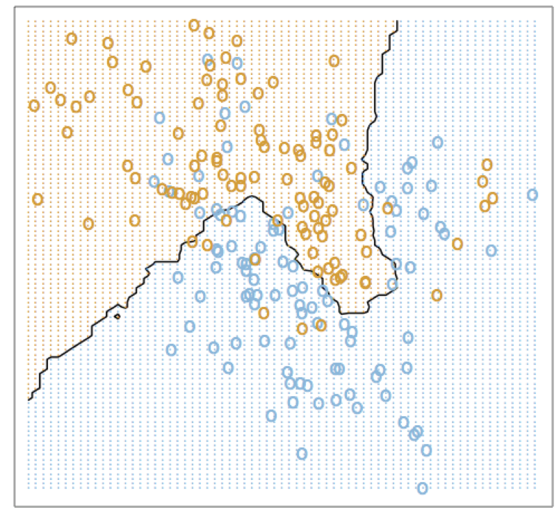
This approach is akin to taking a view opposite to the Bayes classifier: whereas Bayes assumes full knowledge and takes advantage of the data distribution, Nearest neighbors (NN) completely ignores the underlying probability distribution. At a high level, the NN method is based on the belief that features that are used to describe the data are relevant to the labelling in a way that makes “close by” points likely to have the same label.

NN is one of the simplest possible classifiers, where the training process is essentially to memorize the training data. Then during testing, for a given point $x$, it finds the $k$ points in training data nearest to $x$ and predicts a label by taking (weighted) majority label over these $k$ points.

Precisely, given training data \(S=\left\{\left(x_{i}, y_{i}\right), 1 \leq i \leq N\right\},\) the NN prediction rule is defined as:

\[\mathrm{NN}_{k}(x) :=\left\{j | 1 \leq j \leq k, x_{j}\text { is within } k \text { closest to } x\right\}.\]

Note that 1-NN classifier \(\mathrm{NN}_{1}(x)=\operatorname{argmin}_{1 \leq i \leq N} \operatorname{dist}\left(x, x_{i}\right)\). And the $k$-NN classifier \(h_{k\text{-NN}}(x) = \frac{1}{k} \sum_{\ell \in \mathrm{NN}_{k}(x)} y_\ell.\)

k-NN can learn complex nonlinear classifiers (Image Credit: Elements of Statistical Learning Theory)

Nearest Neighbor and Bayes

Despite its simplicity, nearest neighbor is capable of learning complex nonlinear classifiers. Precisely, the risk of nearest neighbor

\[\begin{aligned}L_{k\text{-NN}} & = \mathbb{P}(h_{k\text{-NN}}(X) \neq Y).\end{aligned}\]

NN classifier has excellent asymptotic performance:

Let $\mathcal{X} \subset \mathbb{R}^d, ~d\geq 1$. Let $\eta$ be continuous. Then, \(\begin{aligned}\lim_{n\to\infty} L_{1\text{-NN}} & = 2 \mathbb{E}\big[\eta(X) (1-\eta(X))\big] ~\leq~2 \mathbb{E}\big[\min\{\eta(X), 1-\eta(X)\}] ~=~ 2 L^*. \end{aligned}\)

That is, with large number of data points, $1$-nearest-neighbor algorithm has risk that is within factor $2$ of the optimal risk.

Given $X = x$, let $X’(n)$ be the one closest data point to $x$ amongst given $n$ observations. Then due to $\mathcal{X} \subset \mathbb{R}^d$ (i.e. complete, separable metric space), it can be argued that $X’(n) \to x$ as $n\to \infty$ with probability $1$; further, note that $\eta$ is continuous.

Therefore, $\eta(X’(n)) \to \eta(x)$ as $n\to \infty$ with probability $1$. Let $Y’(n)$ be the label observed associated $X’(n)$. Then,

\[\begin{aligned} \mathbb{P}(h_{1\text{-NN}}(x) \neq Y | X = x) & = \mathbb{P}(Y'(n) \neq Y | X = x) \\ & = \mathbb{P}(Y'(n) = 1, Y = 0| X = x) + \mathbb{P}(Y'(n) = 0, Y = 1| X = x) \\ & \stackrel{(a)}{=} \mathbb{P}(Y'(n) = 1 | X = x) \mathbb{P}( Y = 0 | X = x) \\ & \quad + \mathbb{P}(Y'(n) = 0 | X = x) \mathbb{P}( Y = 1| X = x) \\ & = \eta(X'(n)) (1-\eta(x)) + (1-\eta(X'(n)) \eta(x) \\ & \to 2 \eta(x) (1-\eta(x)) \\ & \stackrel{(b)}{=} 2 \min\{\eta(x), 1-\eta(x)\} \max\{\eta(x), 1-\eta(x)\} \\ & \stackrel{(c)}{\leq} 2 \min\{\eta(x), 1-\eta(x)\}. \end{aligned}\]

In above, (a) follows from the fact that $Y’(n)$ and $Y$ are generated independently per our generative model; (b) from that the fact for \(\alpha, \beta \in \mathbb{R}\) we have \(\alpha \beta = \min\{\alpha, \beta\} \max\{\alpha, \beta\}\); and (c) from the fact that $\eta(x) \in [0,1]$ as it is probability.

Then, the claim of theorem follows by recalling that the Bayes risk $L^* = \mathbb{E}[\min{\eta(X), 1-\eta(X)}]$.

The nearest neighbor approach is powerful in that it works for any (reasonable) setting. Since there are no parameters to be learned, it is called non-parametric method. However, it comes at the cost of not utilizing the potentially simpler, a priori known structure in the data. For that reason, it suffers from requiring large amount of data (there is no ‘free lunch’).

However, if we have prior knowledge about the model class, it may make sense to incorporate it. And this is where the framework of Empirical Risk Minimization through incorporating “inductive bias” comes handy and we describe that next.

Empirical Risk Minimization

ERM makes the following trade-off: we accept that we do not know the full distribution (unlike the Bayes Classifier), but we do get to see the training data and we are not ignoring the training distribution (unlike NN classifiers).

By not throwing away the training distribution, we can at least measure the error incurred by a classifier on the training data, aka the training error or empirical risk:

\[L_{S}(h) :=\frac{1}{N} \big|\left\{i \in[N] | h\left(x_{i}\right) \neq y_{i}\right\} \big|.\]

As the name suggests, the paradigm of Empirical Risk Minimization (ERM) seeks a predictor that minimizes $L_{S}(h)$. In other words, it uses $L_{S}(h)$ as a proxy for the true risk. Notice how this implies that while we do not throw away any “knowledge” gained from the training data, we are implicitly assuming the distribution of the training data is “representative” of the true underlying distribution.

Over-fitting

Of course, greedily minimizing the empirical loss can lead to overfitting. If we get “unlucky” where the training data is not true example of the actual distribution, then over-fitting would lead to high error on unseen data, which is obviously problematic.

Food for thought: What is over-fitting? Essentially it’s fitting the data too well, or memorizing the training data. But is it necessarily bad? In itself not necessarily a bad idea; some argue that deep neural nets are essentially memorizing, yet they generalize well.

Inductive bias

Since it is so easy to overfit when minimizing empirical risk, we search for settings where overfitting can be alleviated. One idea is to introduce the so-called “inductive bias”, which restricts the family of classifiers that we search over; this choice is made in advance before having seen any training data.

Common examples of inductive-bias include linear models, neural networks, random forests, etc. The reason this is called a bias is because we are limiting ourselves to a “pre-determined” hypothesis class that we chose (i.e. our “bias” is present). And by doing so, it may not have any classifier that perfectly fits the data – that is, overfitting is avoided.

Formally, let $\mathrm{ERM}_{\mathcal{H}}$ uses ERM to learn $h : \mathcal{X} \rightarrow \mathcal{Y}$ over $h \in {\cal H}$ by using the training data $S$:

\[\operatorname{ERM}_{\mathcal{H}}(S) \in \underset{h \in \mathcal{H}}{\operatorname{argmin}} L_{S}(h).\]

In other words, we are now minimizing a constrained empirical risk. Ideally, the choice of ${\mathcal{H}}$ should be governed by the knowledge of the data. But even “simple” choices of ${\mathcal{H}}$ can overfit if we are not careful. Of course, overly strong inductive bias can lead to under-fitting. How to balance between the overfit and underfit is precisely the job of machine learning designers.

Loss function, ERM setup

Now let us write the ERM as a mathematical problem. Recall, the (true) risk is defined as

\[L(h)=\mathbb{P}(h(X) \neq Y).\]

Here we introduce a generic framework that encapsulates variety of “risks”. To that end, consider a loss function \(\ell : \mathcal{H} \times \mathcal{X} \times \mathcal{Y} \rightarrow \mathbb{R}_{+}.\) Then, the risk can then be written as the expected loss upon using $h \in \mathcal{H}$ with respect to the data distribution $\mathbb{P},$ that is, \(L(h) :=\mathbb{E}[\ell(h, X, Y)].\)

Similarly, the empirical risk is using $N$ data points is \(L_{S}(h) :=\frac{1}{N} \sum_{i=1}^{N} \ell\left(h, x_{i}, y_{i}\right).\) The classification risk we have considered thus far corresponds to \(0/1\)-loss:

\[\ell_{0 / 1}(h,x, y) :=\left\{\begin{array}{ll}{1,} & {h(x) \neq y} \\ {0,} & {h(x)=y},\end{array}\right.\]

which incurs a loss of $1$ if the current data is mis-classified. When we shall discuss regression, we will introduce different (squared) loss.

Verify that \(\ell_{0 / 1} \text { reduces to } L(h)=\mathbb{P}(h(X) \neq Y).\)

Under the $0/1$-loss, the task of ERM reduces to the computational question:

\[\min _{h \in \mathcal{H}} \frac{1}{N} \sum_{i=1}^N \ell_{0 / 1}\left(h, x_i, y_i\right)=\frac{1}{N} \sum_{i=1}^N \llbracket h\left(x_i\right) \neq y_i \rrbracket\]

This empirical risk minimization is typically computationally hard. One way to get around the computational hardness is to utilize simpler surrogate loss. For example, the so-called support vector machine utilizes the “hinge loss”. In another fundamental classification method, the so-called logistic regression method (as you might have noticed, there’s something quite confusing here, that even though logistic regression has regression in the name, it’s really a classification method), the surrogate to $0-1$ loss is the sigmoid function.

ERM: Theory

The ERM theory asks this question: when does ERM work? In other words, if we minimize the empirical risk $L_{S}(h)$, what bearing does that have on the population risk $L(h)$? The goal of learning theory is to study questions such as this.

Informally, if for all $h \in \mathcal{H},$ the empirical risk $L_{S}(h)$ is a good approximation to $L(h),$ then ERM will also return a good hypothesis within ${\cal H}$, and we may be able to establish a bound of the form

\[L_{\mathbb{P}}\left(\operatorname{ERM}_{\mathcal{H}}(S) \right) \leq \min _{h \in \mathcal{H}} L_{\mathbb{P}}(h) + \varepsilon(n, {\cal H}).\]

where recall that $\operatorname{ERM}_{\mathcal{H}}(S)$ is the classifier learned using ERM; both risks are taken over the data distribution as well as randomly generated $S$ per the data distribution, and $n$ is the number of training data points.

If such is that case, then empirical risk of $\operatorname{ERM}_{\mathcal{H}}(S)$ will provide a good proxy of the best population risk achievable by ${\cal H}$. Naturally, the larger ${\cal H}$ we have, the better the best population risk minimization is achieved over this ${\cal H}.$ So then what stops us from just choosing a very large ${\cal H}$?

ERM: Bias-complexity tradeoff

At a high level, typically for a fixed $n,$ $\varepsilon(n, {\cal H})$ increases with the increase of ${\cal H}$ complexity; and \(\min _{h \in \mathcal{H}} L_{\mathbb{P}}(h)\) decreases as ${\cal H}$ complexity increases. That is, if we increase complexity of ${\cal H}$, then the “bias”, represented via \(\min _{h \in \mathcal{H}} L_{\mathbb{P}}(h)\) decreases. But “variance”, represented via \(\varepsilon(N, {\cal H})\) increases.

Our ultimate goal is to achieve the right trade-off between these two for a given number of data points $n$.

Classical training vs test curve. (Figure taken from: .)

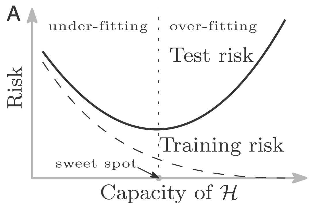
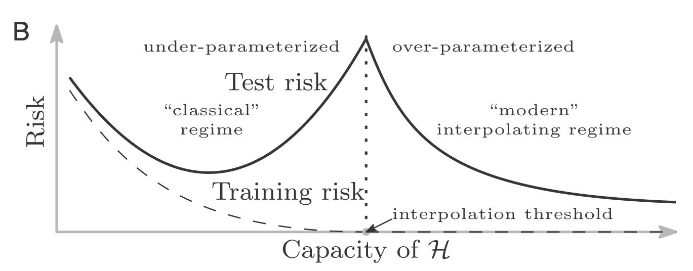
This bias-variance tradeoff or tension is captured by Figure 1. This is the classical view point. In the recent times, practitioners have found “rich” models e.g. over parametrized neural networks and empirically observed that once passed a certain complexity (of the model class $\mathcal{H}$), beyond the so-called interpolation threshold point, the data can be fit perfectly as well as the generalization continues to improve. This is shown by the double-descent curve in Figure 2. It is believed that this behavior is similar to that of non-parametric method like the nearest neighbor that generalizes well for all setting with enough observations even when the corresponding model class is extremely rich.

Modern training vs test curve. (Figure taken from: .)

Extra reading: [SB]/[SSS] Understanding Machine Learning: From Theory to Algorithms, Shalev-Shwartz and Ben-David; Cambridge University Press, 2014:

• Setup/Definitions: §2.1,

• ERM and inductive bias: §2.2, §2.3,

• Loss function: §12.3, §3.2.2,

• Nearest neighbor §19.0, §19.1.