Regression

Table of contents

1. Overview
2. Introduction to Regression
   1. 1-Dimensional Example
3. The Optimal Estimator
4. Linear Least-Squares Regression
   1. Analysis of Linear Least-Squares Regression
5. Non-linear Least-Squares Regression

Overview

This lecture introduces a new machine learning task: regression. In regression the goal is to predict real numbers from features. This is significantly different from classification, where each label represents a category, and where we do not assume any relation between the categories. This lecture will cover ERM formulations of regression, and in particular the least-squares formulation. We will then analyze a linear model for regression and prove that its expected prediction error goes to zero as the number of samples goes to infinity. Finally, we will extend linear regression to allow nonlinear features by developing a kernelized version of linear regression.

Introduction to Regression

Let the training data be $S = {(x_1, y_1), …, (x_N,y_N)}$ where $x_i \in \mathbb{R}^d$, $y_i \in \mathbb{R}$, $\forall i \in {1, …, N}$. The goal is to learn a rule $h: \mathbb{R}^d \to \mathbb{R}$ that can predict the values $y$ from the features $x$.

The most common empirical risk minimization formulation in regression uses the square loss, and is defined as follows:

\[\min_{h \in\mathcal{H}} \frac{1}{N}\sum_{i=1}^N (h(x_i) - y_i)^2.\]

A common class of estimators is the linear one:

\[\mathcal{H} = \{h:\mathbb{R}^d \to \mathbb{R} \big| h(x) = w_0 + w^T x, w_0 \in \mathbb{R}, w \in \mathbb{R}^d\}.\]

The combination of empirical risk minimization with square loss and linear estimators is called linear least-squares regression.

We will develop a more formal view of regression in later sections. For now, we will look at an example of applying linear least-squares regression to the case where $x$ is one-dimensional.

1-Dimensional Example

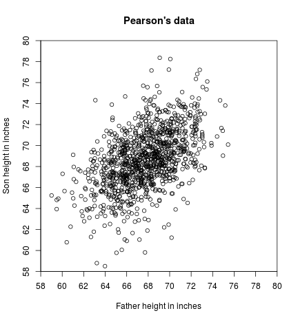
Let ${(x_1, y_1), …, (x_N, y_N)}$ be a set of points, where each point $(x_i, y_i)$ represents the heights of a father ($x_i$) and his son ($y_i$). The goal is to learn a linear model that can predict the height of a son from the height of his father. Figure 1 shows a scatter plot of $1078$ such data points, originally collected by Karl Pearson for a study on the heritability of heights – a very early application of regression.

Scatter Plot of Father’s Heights and Son’s Heights, According to Pearson’s data. Source: https://www.r-bloggers.com/lr01-correlation.

We consider a linear model $y = w_0 + wx$. To obtain an estimate of the coefficients $w_0$ and $w$, we solve the least-squares problem \(\min_{w_0, w} L(w_0, w) = \sum_{i=1}^N(y_i - w_0 - wx_i)^2\) where we dropped the $\frac{1}{N}$ term, which is a constant and does not affect the optimization. The objective is convex in $w_0$ and $w$, so we can find the minimum by taking derivatives and setting them to zero. We have \(\frac{\partial L}{\partial w_0} = -2\sum_{i=1}^N(y_i-w_0-wx_i) = 0,\) \(\frac{\partial L}{\partial w} = -2 \sum_{i=1}^N (y_i-w_0-wx_i) x_i = 0.\) From the form for $\frac{\partial L}{\partial w_0}$, we get that: \(\begin{aligned} &N w_0 = \sum_{i=1}^N y_i - w \sum_{i=1}^N x_i\\ &\Longrightarrow w_0 = \frac{1}{N} \sum_{i=1}^N y_i - w \frac{1}{N} \sum_{i=1}^N x_i \\ &\Longrightarrow w_0 = \overline{y} - w \overline{x} \end{aligned}\) where in the second line we divided by $\frac{1}{N}$, and in the last line we used the notation $\overline{x} = \frac{1}{N}\sum_{i=1}^N x_i$ and $\overline{y} = \frac{1}{N}\sum_{i=1}^N y_i$. From the form for $\frac{\partial L}{\partial w}$, we get that: \(\begin{aligned} &w \sum_{i=1}^N x_i^2 = \sum_{i=1}^N x_iy_i - w_0 \sum_{i=1}^N x_i\\ &\Longrightarrow w \sum_{i=1}^N x_i^2 = \sum_{i=1}^N x_iy_i - (\overline{y} - w\overline{x}) \sum_{i=1}^N x_i\\ &\Longrightarrow w \left( \frac{1}{N} \sum_{i=1}^N x_i^2 - \frac{1}{N} \overline{x} \sum_{i=1}^N x_i \right) = \frac{1}{N} \sum_{i=1}^N x_i y_i - \overline{y} \frac{1}{N} \sum_{i=1}^N x_i\\ &\Longrightarrow w (\overline{x^2} - (\overline{x})^2) = \overline{x \circ y} - \overline{x} \cdot \overline{y}\\ &\Longrightarrow w = \frac{\overline{x \circ y} - \overline{x} \cdot \overline{y}}{\overline{x^2} - (\overline{x})^2} \end{aligned}\) where in the third line we divided by $\frac{1}{N}$, and in the second-to-last line we used the notation $\overline{x^2} = \frac{1}{N} \sum_{i=1}^N x_i^2$ and $\overline{x\circ y} = \frac{1}{N} \sum_{i=1}^N x_i y_i$.

In the limit of infinite data, we can replace the averaged variables (i.e. those with a bar above them) by their expectations. That is, we get: \(w_0 = \mathbb{E}[Y] - w \mathbb{E}[X],\) \(\begin{aligned} w &= \frac{\mathbb{E}[XY] - \mathbb{E}[X]\mathbb{E}[Y]}{\mathbb{E}[X^2] - \mathbb{E}[X]^2} = \frac{\operatorname{cov}(X,Y)}{\sigma_X^2} = \frac{\operatorname{cov}(X,Y)}{\sigma_X \sigma_Y} \left(\frac{\sigma_Y}{\sigma_X}\right) \end{aligned}\) where we use $\operatorname{cov}(X,Y) = \mathbb{E}[(X-\mathbb{E}[X])(Y-\mathbb{E}[Y])] = \mathbb{E}[XY] - \mathbb{E}[X]\mathbb{E}[Y]$ to denote the covariance of $X$ and $Y$, and $\sigma_X^2 = \mathbb{E}[(X-\mathbb{E}[X])^2] = \mathbb{E}[X^2] - \mathbb{E}[X]^2$ to denote the variance of $X$ (and similarly for $Y$). In particular, the term \(r(X,Y)=\frac{\operatorname{cov}(X,Y)}{\sigma_X \sigma_Y}\) is called the Pearson correlation of $X$ and $Y$.

The Optimal Estimator

The previous example found an ERM solution for a class of linear models. But our actual goal is to find a good estimator $h: \mathcal{X} \to \mathcal{Y}$ for the entire data distribution. At the population level (i.e. with infinite data), the problem becomes one of minimizing the expected square loss: \(\min_{h} \mathbb{E}_{X,Y}[(h(X)-Y)^2].\) In this formulation, what is the best estimator $h$ to use? It turns out that the best estimator is always \(h(x) = \eta(x) = \mathbb{E}[Y|X=x].\) This estimator is analogous to the Bayes classifier in classification tasks. We prove in Theorem 1 that $\eta$ is the estimator with the lowest expected square loss.

*Let $\eta(x) = \mathbb{E}[Y|X=x]$ and let $h : \mathbb{R}^d \to \mathcal{Y}$. Then $$\mathbb{E}[(\eta(X)-Y)^2] \leq \mathbb{E}[(h(X)-Y)^2].$$

For each $x \in \mathbb{R}^d$ we have: $$\begin{aligned} \mathbb{E}[(h(X)-Y)^2|X=x] &= \mathbb{E}[(h(X)-\eta(X)+\eta(X)-Y)^2|X=x]\\ &= \mathbb{E}[(h(X)-\eta(X))^2|X=x] + \mathbb{E}[(\eta(X)-Y)^2|X=x]\\ &\qquad + 2 \mathbb{E}[(h(X)-\eta(X))(\eta(X)-Y)|X=x]\\ &= \mathbb{E}[(h(X)-\eta(X))^2|X=x] + \mathbb{E}[(\eta(X)-Y)^2|X=x]\\ &\qquad + 2 (h(x)-\eta(x)) \mathbb{E}[\mathbb{E}[Y|X=x]-Y|X=x]\\ &= \mathbb{E}[(h(X)-\eta(X))^2|X=x] + \mathbb{E}[(\eta(X)-Y)^2|X=x]\\ &\geq \mathbb{E}[(\eta(X)-Y)^2|X=x] \end{aligned}$$ All that is left is to integrate/add over all values of $x$ (depending on the domain $\mathcal{X}$). Assuming a continuous domain on which the probability density function of $X$ at $x$ is $p_X(x)$: $$\begin{aligned} &\mathbb{E}[(\eta(X)-Y)^2|X=x] \leq \mathbb{E}[(h(X)-Y)^2|X=x]\\ &\Longrightarrow \int_x \mathbb{E}[(\eta(X)-Y)^2|X=x] p_X(x) dx \leq \int_x \mathbb{E}[(h(X)-Y)^2|X=x] p_X(x) dx\\ &\Longrightarrow \mathbb{E}[\mathbb{E}[(\eta(X)-Y)^2|X]] \leq \mathbb{E}[\mathbb{E}[(h(X)-Y)^2|X]]\\ &\Longrightarrow \mathbb{E}[(\eta(X)-Y)^2] \leq \mathbb{E}[(h(X)-Y)^2] \end{aligned}$$ 

However, we usually do not know the joint probability distribution $\mathbb{P}(X,Y)$, so we cannot use $\mathbb{E}[Y|X=x]$ as our estimator. Therefore, similarly to classification, we will assume some functional form for $\mathbb{E}[Y|X=x]$ and learn it from data.

Linear Least-Squares Regression

In linear regression, we assume \(\mathbb{E}[Y|X=x] = w^Tx+w_0,\) or, with non-linear features, \(\mathbb{E}[Y|X=x] = w^T\phi(x)+w_0.\) For now, we will focus on the case with linear features. The goal is to minimize the risk: \(\min_{w,w_0} \mathbb{E}[l(w^Tx+w_0, y)].\) The corresponding ERM strategy is: \(\min_{w,w_0} \frac{1}{N} \sum_{i=1}^N l(w^Tx_i + w_0, y).\) We typically use the square loss: \(l(\hat{y},y) = \frac{1}{2}(y-\hat{y})^2.\)

In what follows, we will ignore the intercept term $w_0$. Note that an easy way to incorporate it into the problem is to add one coordinate that is always $1$ to each data point $x$. Then the term in $w$ corresponding to that coordinate plays the role of $w_0$.

We can now write out the complete formulation of the problem. Given training data $S={(x_1, y_1), …, (x_N, y_N)}$ where $x_i\in\mathbb{R}^d$, $y_i\in\mathbb{R}$, we minimize: \(\min_{w} L(w) = \min_w \sum_{i=1}^N (y_i-w^Tx_i)^2 = ||Xw-y||^2\) where $X \in \mathbb{R}^{N\times d}$, $y \in \mathbb{R}^N$, $w \in \mathbb{R}^d$.

Note that we also dropped the $\frac{1}{N}$, as it does not affect the optimization.

To find the optimal value of $w$, we calculate the gradient of $L$ with respect to $w$ and set it to $0$: \(L(w) = (Xw-Y)^T(Xw-Y) = w^TX^TXw + y^Ty - 2w^TX^Ty\) \(\begin{aligned} &\nabla_w L(w) = 2X^TXw - 2X^Ty = 0\\ &\Longrightarrow w = (X^TX)^{-1}X^Ty \end{aligned}\)

Note that, if we have nonlinear features, we get $w = (\Phi^T \Phi)^{-1}\Phi^T y$.

Question: What happens to the solution if $d < N$? What if $d > N$?

Answer: The relevant term is $X^TX$, which we need to be invertible. This term has dimensionality $d\times d$. The case $d < N$ is not problematic, because $X^TX$ will be full-rank as long as the rank of $X$ is $d$. However, in the case $d > N$, $X^TX$ cannot be full-rank, as this would imply the rank of $X$ is $d$, which is impossible. Therefore, $X^TX$ is not invertible. In this case, we typically use the pseudoinverse instead of the inverse: $w = (X^TX)^\dagger X^T y$, where the $\dagger$ symbol denotes the pseudoinverse.

Analysis of Linear Least-Squares Regression

Assume that the true underlying model is linear: \(y = w_{true}^T x.\) Does solving least-squares work in this case? Does it recover $w_{true}$? There are some difficulties in answering this question. In particular, our concepts of learnability and VC-dimension were limited to binary classification. In regression, we need a different framework. A widely used idea to analyze regression is that of Rademacher complexity ( §26). However, these ideas go beyond the scope of this class.

We will look instead at an empirical observation model, in which we will analyze what happens as the number of data points increases. Assume the model: \(y = w^T x+ \eta, \qquad \eta \sim N(0, \sigma^2).\) Thus, the data points satisfy \(y_i = w^T x_i + \eta_i, \qquad \eta_i \sim N(0, \sigma^2).\) In this model, we observe the true $x_i$ and the corresponding noisy $y_i$. The parameter $w$ is unknown. We estimate $w$ by some $\hat{w}$ which we obtain by solving the least-squares problem.

Note that, after estimating $\hat{w}$, we make predictions $\hat{y}_i = \hat{w}^T x_i$. We want to analyze the error of these empirical predictions from the true expected predictions. This error is \(\frac{1}{N} \sum_{i=1}^N (\hat{y}_i - \mathbb{E}[y_i])^2 = \frac{1}{N} ||X\hat{w}-Xw||\) where we used that $\hat{y}_i = \hat{w}^T x_i$ and $\mathbb{E}[y_i] = \mathbb{E}[w^T x_i + \eta_i] = w^T x_i$. Theorem 2 shows that this error goes to $0$ as the number of data points goes to infinity.

(Informal) *$$\lim_{N \to \infty} \mathbb{E}\left[ \frac{1}{N} ||X\hat{w}-Xw||^2 \right] = 0$$*

The expectation in Theorem 2 is over the noise in the observations. We will now prove the theorem.

*Proof.* Note that $\hat{w} = \mathop{\mathrm{argmin}}_\theta ||X\theta-y||^2 = (X^TX)^{-1}X^Ty$. We have: $$\begin{aligned} ||X\hat{w}-Xw||^2 &= ||X\hat{w} - y + \eta||^2 & [\text{uses } y=Xw+\eta]\\ &= ||X\hat{w}-y||^2 + ||\eta||^2 + 2 \eta^T(X\hat{w}-y)&\\ &\leq ||Xw-y||^2 + ||\eta||^2 + 2 \eta^T(X\hat{w}-y) & [\text{uses } \hat{w}=\mathop{\mathrm{argmin}}_\theta ||X\theta-y||^2]\\ &= ||Xw-y||^2 + ||\eta||^2 + 2 \eta^T(X\hat{w}-Xw-\eta)&\\ &= ||\eta||^2 + ||\eta||^2 + 2 \eta^T(X\hat{w}-Xw) - 2||\eta||^2&\\ &= 2 \eta^T X\hat{w}-2\eta^T Xw& \end{aligned}$$ Note that so far the argument has been deterministic. We take now expectations over $\eta$, noting that $\mathbb{E}[\eta] = 0$ and that $\eta$ is independent of $Xw$. So: $$\begin{aligned} \mathbb{E}[||X\hat{w}-Xw||^2] &\leq 2 \mathbb{E}[\eta^T X\hat{w}]-2\mathbb{E}[\eta^T Xw]&\\ &= 2 \mathbb{E}[\eta^T X\hat{w}]&[\text{uses } \mathbb{E}[\eta]=0]\\ &= 2 \mathbb{E}[\eta^T X(X^TX)^{-1}X^Ty]&\\ &= 2 \mathbb{E}[\eta^T X(X^TX)^{-1}X^T(Xw+\eta)]&\\ &= 2 \mathbb{E}[\eta^T X(X^TX)^{-1}X^TXw] + 2 \mathbb{E}[\eta^T X(X^TX)^{-1}X^T\eta]&\\ &= 2 \mathbb{E}[\eta^T Xw] + 2 \mathbb{E}[\eta^T X(X^TX)^{-1}X^T\eta]&\\ &= 2 \mathbb{E}[\eta^T X(X^TX)^{-1}X^T\eta] & [\text{uses } \mathbb{E}[\eta]=0]\\ &= 2 \mathbb{E}[\eta^T Q \eta]& \end{aligned}$$ where we define $Q = X(X^TX)^{-1}X^T$. Observe that $\eta^T Q \eta$ is just a scalar, so it is equal to $\operatorname{trace}(\eta^T Q \eta)$. Then, by the property that $\operatorname{trace}(ABC) = \operatorname{trace}(BCA) = \operatorname{trace}(CAB)$, we have $\operatorname{trace}(\eta^TQ\eta) = \operatorname{trace}(Q\eta \eta^T)$. Then: $$\begin{aligned} \mathbb{E}[||X\hat{w}-Xw||^2] &\leq 2 \mathbb{E}[\eta^T Q \eta] = 2 \mathbb{E}[\operatorname{trace}(Q\eta\eta^T)] = 2 \operatorname{trace}(\mathbb{E}[Q\eta\eta^T])\\ &= 2 \operatorname{trace}(Q \mathbb{E}[\eta\eta^T]) = 2 \operatorname{trace}(Q \sigma^2 I_N) = 2 \sigma^2 \operatorname{trace}(Q). \end{aligned}$$ Now we substitute the value of $Q$ back in: $$\begin{aligned} \mathbb{E}[||X\hat{w}-Xw||^2] &\leq 2 \sigma^2 \operatorname{trace}(Q) = 2 \sigma^2 \operatorname{trace}(X(X^TX)^{-1}X^T)\\ &= 2 \sigma^2 \operatorname{trace}((X^TX)^{-1}X^TX) = 2 \sigma^2 \operatorname{trace}(I_d) = 2 \sigma^2 d. \end{aligned}$$ Overall we have: $$0 \leq \mathbb{E}\left[ \frac{1}{N} ||X\hat{w}-Xw||^2 \right] \leq \frac{2\sigma^2d}{N},$$ $$\lim_{N\to\infty} \mathbb{E}\left[ \frac{1}{N} ||X\hat{w}-Xw||^2 \right] = 0.$$ ◻

If $X^TX$ is not invertible, we need to bound $\operatorname{trace}((X^TX)^\dagger X^TX)$, where the $\dagger$ symbol denotes the pseudoinverse. This is still possible, but it is beyond the scope of this class.

Non-linear Least-Squares Regression

With non-linear features, we assume that $\mathbb{E}[Y|x=x] = w^T \phi(x) + w_0$. Then the corresponding ERM strategy with square loss is: \(\min_w L(w) = \min_w \sum_{i=1}^N (y_i-w^T\phi(x_i))^2 = ||\Phi w-y||^2.\) What if $\phi(x)$ has large dimensionality, or is infinite-dimensional? As in the case of classification, this can be accommodated with the use of kernels.

We will look at a formulation called kernelized ridge regression (KRR), in which we also add a regularization term which ensures that there are no issues if the kernel matrix $K$ is not invertible. We define \(\min_w L(w) = \min_w \frac{1}{N} \sum_{i=1}^N (y_i - w^T \phi(x_i))^2 + \lambda ||w||^2.\) Taking the gradient with respect to $w$ and setting it to $0$, we get: \(\lambda w - \frac{1}{N} \sum_{i=1}^N (y_i - w^T \phi(x_i))\phi(x_i) = 0.\) Let us introduce variables $\alpha_i$ such that $N \lambda \alpha_i = y_i - w^T \phi(x_i)$. Then the expression obtained by setting the gradient to $0$ becomes \(\begin{aligned} \lambda w - \lambda \sum_{i=1}^N \alpha_i \phi(x_i) = 0 \Longrightarrow w = \sum_{i=1}^N \alpha_i \phi(x_i). \end{aligned}\) With this representation of $w$, for a new data point $x$ we can calculate the prediction as \(w^T \phi(x) = \sum_{i=1}^N \alpha_i \phi(x_i)^T \phi(x) = \sum_{i=1}^N \alpha_i k(x_i, x)\) Of course, we still need a way to calculate the values $\alpha$. We have: \(N\lambda \alpha_i = y_i - w^T \phi(x_i) = y_i - \sum_{j=1}^N \alpha_j \phi(x_j)^T \phi(x_i) = y_i - \sum_{j=1}^N \alpha_j k(x_j,x_i)\) where we substituted $w$ with its representation in terms of $\alpha$. Then, the expression above in vector form is: \(\begin{aligned} N \lambda \alpha = y - K \alpha \Longrightarrow \alpha = (K+N\lambda I)^{-1}y \end{aligned}\) where $K_{ij}=\phi(x_i)^T\phi(x_j)$. Therefore, it is possible to fully kernelize linear regression.