Regularization
Table of contents
- Overview
- Introduction to Regularization
- The Bias-Variance Tradeoff
- Ridge Regression and The Bias-Variance Tradeoff
- LASSO Regression
- Bayesian View on Regression
Overview
This lecture explores additional views on regression, with a focus on regularization. First, we express the bias-variance tradeoff, in which the loss decomposes into noise, bias, and variance. This formulation will lead us to a possible strategy for lowering the loss: increasing the bias while lowering the variance. We will see how we can think of ridge regression and LASSO regression in terms of the bias-variance tradeoff. Finally, we will look at a Bayesian perspective of regularization in regression.
Introduction to Regularization
Why would one need regularization? The following are some situations in which regularization can be useful:
-
Recall from last lecture that the solution to the linear least-squares problem is $w= (X^TX)^{-1}y$. If $d > N$, $X^TX$ is no longer invertible.
-
Even if $d \leq N$, $X^TX$ may be ill-conditioned. For example, it may have some very small eigenvalues, which will make its inverse blow up, leading to numerical issues.
-
The model may overfit the training data. This is particularly likely if we use non-linear features that are too powerful. Then, the model may not generalize well.
-
We may have some prior knowledge about what the model parameters look like or what the model parameters should look like. Then we may like to impose constraints or penalties to prefer that structure.
Regularization can help with all of these issues! How does one actually use regularization? A common way is to add a regularizer to the empirical risk function, \(\min_w \frac{1}{N} \sum_{i=1}^N (y_i-w^Tx)^2 + \lambda\Omega(w)\) for some $\lambda > 0$ and some function $\Omega$. The role of $\lambda$ is to assign a weight to the regularizer, relative to the squared loss. Note that as $\lambda \to 0$, we return to the non-regularized version studied in the previous lecture.
Why does regularization help? Regularization reduces the effective capacity (or complexity) of the model, which can help it generalize better. In classification, this topic is studied through Structural Risk Minimization theory.
Note that regularization does not need to be explicit, as in the example above. Regularization can be achieved implicitly, through the choice of model, algorithm, computation, data augmentation, and several other strategies.
The Bias-Variance Tradeoff
We will now explore the bias-variance tradeoff, which provides useful insights into how regularization works. Consider the noisy observation model from last lecture: \(y = f(x)+\eta\) where $y \in \mathbb{R}$, $x \in \mathbb{R}^d$, $\eta \sim N(0, \sigma^2)$. For this part of the lecture, $f$ does not need to be linear. We solve the least-squares problem to come up with a predictor $\hat{f}$. The expected error of our predictor on a new data point is: \(\mathbb{E}[(y-\hat{y})^2]=\mathbb{E}[(y-\hat{f})^2]\) where $y$ is the label of the new data point, and $\hat{y} = \hat{f}$ is the label predicted for the new data point, using the $\hat{f}$ learned from the training set. The expectation is over the noise in the training set and the noise in the observation of the new data point.
The the bias-variance tradeoff refers to the following equality, which decomposes the expected error in three terms: \(\begin{aligned} \mathbb{E}[(y - \hat{f})^2] &= \mathbb{E}[\eta^2] &\text{(noise)}\\ &+ \mathbb{E}[(f - \mathbb{E}\hat{f})^2] &(\text{bias}^2)\\ &+ \mathbb{E}[(\hat{f} - \mathbb{E}\hat{f})^2] &\text{(variance)} \end{aligned}\)
where $\eta$ is the noise of the new data point. The term $\mathbb{E}[\eta^2]$ is inevitable, and comes from the inherent noise in the observation model. The term $\mathbb{E}[(f-\mathbb{E}\hat{f})^2]$ is a bias term, as it quantifies how the average value of $\hat{f}$ differs from the true $f$. The term $\mathbb{E}[(\hat{f}-\mathbb{E}\hat{f})^2]$ is a variance term, as it quantifies how $\hat{f}$ differs from the average value of $\hat{f}$.
We prove now the bias-variance tradeoff equality.
\[\begin{aligned} \mathbb{E}[(y-\hat{f})^2] &= \mathbb{E}[(y-f+f-\hat{f})^2]&\\ &= \mathbb{E}[(y-f)^2]+\mathbb{E}[(f-\hat{f})^2]+2\mathbb{E}[(y-f)(f-\hat{f})]&\\ &= \mathbb{E}[\eta^2]+\mathbb{E}[(f-\hat{f})^2]+2\mathbb{E}[\eta(f-\hat{f})]&\\ &= \mathbb{E}[\eta^2]+\mathbb{E}[(f-\hat{f})^2]&\\ &= \mathbb{E}[\eta^2] + \mathbb{E}[(f - \mathbb{E}\hat{f} + \mathbb{E}\hat{f} - \hat{f})^2]&\\ &= \mathbb{E}[\eta^2] + \mathbb{E}[(f - \mathbb{E}\hat{f})^2] + \mathbb{E}[(\mathbb{E}\hat{f} - \hat{f})^2] + 2 (f - \mathbb{E}\hat{f})^T \mathbb{E}[\mathbb{E}\hat{f} - \hat{f}]&\\ &= \mathbb{E}[\eta^2] + \mathbb{E}[(f - \mathbb{E}\hat{f})^2] + \mathbb{E}[(\mathbb{E}\hat{f} - \hat{f})^2] & [\text{uses } \mathbb{E}[\mathbb{E}\hat{f} - \hat{f}] = 0] \end{aligned}\]We can now look at linear regression from the perspective of the bias-variance tradeoff. Theorem 1 shows that linear regression achieves the smallest expected error among all unbiased linear estimator.
The linear least-squares estimator is the best unbiased linear estimator (i.e. the lowest variance estimator among linear estimators).
This theorem leaves open the possibility of achieving smaller expected error with linear estimators, as long as they are biased. Such estimators would need to increase the bias but reduce the variance, and overall reduce the expected error.
In general, increasing the model complexity leads to higher variance (fits noise more exactly) and lower bias (fits true model more exactly). Conversely, decreasing the model complexity leads to lower variance and higher bias.
In linear regression, we can think of the model complexity as the set of feasible parameters $w$. We can achieve a bias-variance tradeoff by changing the restrictions on this set. For example, one could add a regularizer and use the $\lambda$ parameter to tune the bias and the variance. See Figure 1 for a plot of these quantities for the problem of minimizing \(\frac{1}{N}||Xw-y||^2+\lambda||w||^2.\) Note that, in this case, there exists an optimal value of $\lambda$ that achieves the best tradeoff.

Ridge Regression and The Bias-Variance Tradeoff
We will now show that ridge regression, which uses an $l_2$ regularizer, is biased. Then, we will compute the bias and variance terms for the more general case of kernel ridge regression.
Recall that in ridge regression the objective is \(\min_w \frac{1}{N} \sum_{i=1}^N (y_i - w^T x_i)^2 + \lambda ||w||^2\) and the corresponding solution is \(w = (X^T X + N \lambda I)^{-1}X^T y.\) Note that the term $N\lambda I$, added by the regularizer, makes $X^T X + N \lambda I$ invertible, because it increases all the eigenvalues of the positive semidefinite matrix $X^TX$ by $N \lambda$. This effect was the original motivation for ridge regression in .
We will now prove that the ridge regression solution is biased. For ease of notation, let $M = X^TX$. We have: \(\begin{aligned} w &= (M + N\lambda I)^{-1}X^T y\\ &= [M(I+N\lambda M^{-1})]^{-1}M[M^{-1}X^T y]\\ &= (I + N \lambda M^{-1})^{-1}M^{-1}M w_{ls}\\ &= (I + N \lambda M^{-1})^{-1} w_{ls} \end{aligned}\) where $w_{ls}$ is the least-squares solution (without regularization). What remains to prove is that the least-squares solution is unbiased; i.e. that $\mathbb{E}[w_{ls}]= w_{true}$. (Recall that we are using the observation model $y=Xw_{true}+\eta$.) This clearly implies that $\mathbb{E}[w] \neq w_{true}$ for any $\lambda > 0$. We have: \(\begin{aligned} \mathbb{E}[w_{ls}] &= \mathbb{E}[(X^TX)^{-1}X^Ty]&\\ &= \mathbb{E}[(X^TX)^{-1}X^T(Xw_{true}+\eta)]&\\ &= (X^TX)^{-1}X^TXw_{true}+\mathbb{E}[(X^TX)^{-1}X^T\eta]&\\ &= (X^TX)^{-1}X^TXw_{true}&\\ &= w_{true}. \end{aligned}\)
We will now look at kernel ridge regression and write the bias and variance in a closed form. In this case, the observation model over $N$ data points is \(y = w^T \phi(x) + \epsilon, \qquad \epsilon \sim N(0, C)\) where $y \in \mathbb{R}^N$, $\epsilon \in \mathbb{R}^N$. Note that the noise can be correlated. Let $z = \mathbb{E}[y]$ and $\hat{z} = K(K+N\lambda I)^{-1}y$. Note that $\hat{z}$ is the prediction made on these points using the kernelized least-squares estimator. Then the expected error minus the noise component is:
\[\begin{aligned} \frac{1}{N}\mathbb{E}[||z-\hat{z}||^2] &= \frac{1}{N}\mathbb{E}[||z-\mathbb{E}\hat{z}||^2] + \frac{1}{N} \mathbb{E}[||\mathbb{E}\hat{z} - \hat{z}||^2] + \frac{1}{N} (z-\mathbb{E}\hat{z})^T\mathbb{E}[\mathbb{E}\hat{z} - \hat{z}]\\ &= \frac{1}{N}\mathbb{E}[||z-\mathbb{E}\hat{z}||^2] + \frac{1}{N} \mathbb{E}[||\mathbb{E}\hat{z} - \hat{z}||^2]\\ &= \frac{1}{N} ||z-\mathbb{E}\hat{z}||^2 + \frac{1}{N} \operatorname{trace}[ \operatorname{var}(\hat{z})]\\ &= \frac{1}{N} ||(I-K(K+N\lambda I)^{-1})z||^2 + \frac{1}{N} \operatorname{trace}[\operatorname{var} (K(K+N\lambda I)^{-1}y)]\\ &= \frac{1}{N} ||((K+N\lambda I)(K+N\lambda I)^{-1} - K(K+N\lambda I)^{-1})z||^2 \\ &\qquad + \frac{1}{N} \operatorname{trace}[(K(K+N\lambda I)^{-1}) \operatorname{var}(y) (K(K+N\lambda I)^{-1})^T]\\ &= \frac{1}{N} ||N\lambda (K+N\lambda I)^{-1}z||^2 + \frac{1}{N} \operatorname{trace} [C (K+N\lambda I)^{-1}K^2(K+N\lambda I)^{-1}]\\ &= N \lambda^2 z^T (K+N\lambda I)^{-2} z + \frac{1}{N} \operatorname{trace} [C (K+N\lambda I)^{-1}K^2(K+N\lambda I)^{-1}] \end{aligned}\]Then the bias is \(N \lambda^2 z^T (K+N\lambda I)^{-2} z\) and the variance is \(\frac{1}{N} \operatorname{trace}[C (K+N\lambda I)^{-1}K^2(K+N\lambda I)^{-1}].\)
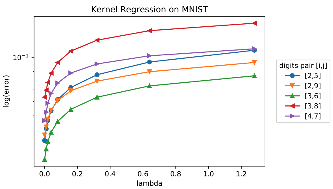
Food for thought: The paper shows a setting in which the best error for kernel ridge regression is obtained by setting $\lambda \approx 0$. See Figure 2. Is this a violation of the bias-variance tradeoff?
LASSO Regression
In general, an $l_p$ regularizer leads to the objective \(\min_w \frac{1}{N} \sum_{i=1}^N (y_i - w^Tx_i)^2 + \lambda ||w||_p^p.\) For $p=2$, we get ridge regression. For $p=1$, we get LASSO.
Note that there are many other choices of regularizer; these include the nuclear norm, the atomic norm, and many others.
Food for thought: Which regularizer should we use? When? Why?
LASSO stands for Least Absolute Shrinkage and Selection Operator. LASSO performs automatic selection of relevant features in the data, by encouraging sparsity in the weight vector $w$. LASSO is useful when there is a large number of features that capture a complex model, but the data is limited and does not allow using all these features meaningfully. Ridge regression typically assigns some non-zero weight to each feature. In contrast, LASSO tries to choose the sparsest weight vectors.
As a simple example of the effect of the $l_1$ norm, consider the one-dimensional objective $\min_w (y-w)^2$. With $l_2$ regularization, we get: \(\mathop{\mathrm{argmin}}_w (y-w)^2 + \lambda w^2 = \frac{y}{1+\lambda}.\) In contrast, with $l_1$ regularization, we get: \(\mathop{\mathrm{argmin}}_w (y-w)^2 + \lambda |w| = \begin{cases} y-\frac{\lambda}{2} & \text{if } y > \frac{\lambda}{2}\\ y+\frac{\lambda}{2} & \text{if } y < -\frac{\lambda}{2}\\ 0 & \text{if } y \in \left[-\frac{\lambda}{2}, \frac{\lambda}{2}\right] \end{cases}\) So LASSO performs “thresholding”, such that the smallest values are pushed to zero. Because of this property, it is widely used to obtain sparse solutions.
Bayesian View on Regression
Recall that so far we have been modeling $\mathbb{P}(Y|X=x)$ directly, assuming a linear model with noise. The model we used most often was \(y = w^Tx + \eta, \qquad \eta \sim N(0,\sigma^2).\) Let us try to find the maximum likelihood estimator of $w$ for this model. Suppose we are given training data $S={(x_1, y_1), …, (x_N, y_N)}$, where $x\in \mathbb{R}^d$, $y\in\mathbb{R}$. Then we have: \(\begin{aligned} w &= \mathop{\mathrm{argmax}}_w \prod_{i=1}^N \mathbb{P}(y_i|x_i,w) = \mathop{\mathrm{argmax}}_w \sum_{i=1}^N \log \mathbb{P}(y_i|x_i,w)\\ &= \mathop{\mathrm{argmax}}_w -\sum_{i=1}^N (y_i - w^T x_i)^2 = \mathop{\mathrm{argmin}}_w \sum_{i=1}^N (y_i - w^T x_i)^2 \end{aligned}\) where we used the pdf of the Gaussian and ignored terms that did not depend on $w$. Note that this is the same as the least-squares problem!
Because maximum likelihood estimation can suffer from overfitting, a general question is: how can we encode “prior knowledge or preference” for the model parameters? Previously, we used regularization. Now, we will consider an alternative concept.
Instead of only modeling $\mathbb{P}(Y|X=x)$, we will now “integrate” over the entire family of linear models, incorporating some prior knowledge we may have (or we may wish to enforce) on the parameters. We will model a prior distribution over the parameters, and use it to compute a posterior distribution over the parameters: \(\mathbb{P}(\rm{parameters}|\rm{data}) \propto \mathbb{P}(\rm{data}|\rm{parameters}) \times \mathbb{P}(\rm{parameters}).\) Suppose again we have the data $S={(x_1, y_1), …, (x_N, y_N)}$. We assume the following model: \(\mathbb{P}(S|w) \propto \exp\left(- \frac{1}{2\sigma^2} ||y-Xw||^2\right)\) \(\mathbb{P}(w) \propto \exp\left(-\frac{1}{2} (w-\mu_0)^T S_0^{-1} (w-\mu_0)\right)\) The form for $\mathbb{P}(S|w)$ is obtained by assuming $\mathbb{P}(Y|X=x)$ is modeled as $N(w^Tx, \sigma^2)$, which is the same as before. The important difference is that now we are assuming a probability distribution over $w$.
With these assumptions, we can now compute the posterior distribution over the model parameters: \(\begin{aligned} \mathbb{P}(w|S) &\propto \exp\left(- \frac{1}{2\sigma^2} ||y-Xw||^2\right) \exp\left(-\frac{1}{2} (w-\mu_0)^T S_0^{-1} (w-\mu_0)\right)\\ &\propto \exp\left(- \frac{1}{2\sigma^2} ||y-Xw||^2-\frac{1}{2} (w-\mu_0)^T S_0^{-1} (w-\mu_0)\right)\\ &\propto \exp\left( -\frac{1}{2} w^T J w + h^T w \right) \end{aligned}\) for the choice of $J$ and $h$ as: \(J = S_0^{-1} + \sigma^{-2}X^TX\) \(h = S_0^{-1}\mu_0 + \sigma^{-2}y^TX.\)
If we want to convert back to the form of a multivariate Gaussian, we get that $\mathbb{P}(w|S)$ is a multivariate Gaussian with mean $\mu_N$ and covariance matrix $S_N$, where: \(S_N^{-1} = S_0^{-1} + \sigma^{-2} X^TX\) \(\mu_N = S_N(S_0^{-1}\mu_0 + \sigma^{-2}y^T X).\)
As an example, let $\mu_0=0$, $S_0=s^2I$. Then: \(S_N^{-1} = s^{-2}I+\sigma^{-2}X^TX\) \(\mu_N = \left(\frac{\sigma^2}{s^2}I + X^TX\right)^{-1}y^TX\) The corresponding log-posterior for this choice of $\mu_0$ and $S_0$ is: \(\log \mathbb{P}(w|S) = - \frac{1}{2\sigma^2}||y-Xw||^2-\frac{1}{2s^2}w^Tw + \rm{const}.\) Therefore, maximizing the posterior is the same as solving ridge regression! Therefore, a Gaussian prior on $w$ leads to ridge regression. Other choices of priors on $w$ will lead to other forms of regularized regression (e.g. a Laplace prior will lead to LASSO).
We have seen that a prior distribution on $w$ leads to a posterior distribution over $w$. In addition, this framework provides a predictive distribution for a new data point $x$. We can compute: \(\begin{aligned} \mathbb{P}(y|x, S) = \int_w \mathbb{P}(y|x,w) \mathbb{P}(w|S) dw. \end{aligned}\)
This allows us, for example, not only to predict, but to give a level of confidence for our predictions.
An Experiment
We will show now experimentally how the distribution of $w$ is updated in a simple setting. This example is taken from §3 in . Let $x_i$ be sampled uniformly in $[-1, 1]$. Let $y_i = a_0 + a_1 x_i + \epsilon_i$, where $a_0 = -0.3$, $a_1 = 0.5$, $\epsilon_i \sim N(0, 0.2^2)$. We consider the weight vector $w=(w_0, w_1)^T$ with prior distribution $w \sim N(0, 0.5I)$. Then, Figure 3 shows the distribution on $w$ and six sample lines drawn from it after $0$ samples (i.e. prior), $1$ sample, $2$ samples, and $20$ samples.
Extra reading:
-
Detailed notes on linear regression:
https://www.fm.mathematik.uni-muenchen.de/teaching/teaching_ws1213/lectures/regression/notes.pdf. -
§3 in .
-
Lecture slides on ridge versus LASSO regression:
http://statweb.stanford.edu/~tibs/sta305files/Rudyregularization.pdf -
Sections on regression and LASSO in .